Programming with R
Addressing data
Learning Objectives {.objectives}
- Understand the 3 different ways R can address data inside a data frame.
- Combine different methods for addressing data with the assignment operator to update subsets of data
R is a powerful language for data manipulation. There are 3 main ways for addressing data inside R objects.
- By index (slicing)
- By logical vector
- By name (columns only)
Lets start by loading some sample data:
dat <- read.csv(file = 'data/sample.csv', header = TRUE, stringsAsFactors = FALSE)
Tip {.callout}
The first row of this csv file is a list of column names. We used the header=TRUE argument to
read.csvso that R can interpret the file correctly. We are using the stringsAsFactors=FALSE argument to override the default behaviour for R. Using factors in R is covered in a separate lesson.
Lets take a look at this data.
class(dat)
[1] "data.frame"
R has loaded the contents of the .csv file into a variable called dat which is a data frame.
dim(dat)
[1] 100 9
The data has 100 rows and 9 columns.
head(dat)
      ID Gender      Group BloodPressure  Age Aneurisms_q1 Aneurisms_q2
1 Sub001      m    Control           132 16.0          114          140
2 Sub002      m Treatment2           139 17.2          148          209
3 Sub003      m Treatment2           130 19.5          196          251
4 Sub004      f Treatment1           105 15.7          199          140
5 Sub005      m Treatment1           125 19.9          188          120
6 Sub006      M Treatment2           112 14.3          260          266
  Aneurisms_q3 Aneurisms_q4
1          202          237
2          248          248
3          122          177
4          233          220
5          222          228
6          320          294
The data is the results of an (not real) experiment, looking at the number of aneurisms that formed in the eyes of patients who undertook 3 different treatments.
Addressing by Index
Data can be accessed by index. We have already seen how square brackets [ can be used to subset (slice) data. The generic format is dat[row_numbers,column_numbers].
Challenge - Selecting values 1 {.challenge}
What will be returned by
dat[1,1]?
dat[1,1]
[1] "Sub001"
If we leave out a dimension R will interpret this as a request for all values in that dimension.
Challenge - Selecting values 2 {.challenge}
What will be returned by
dat[,2]?
The colon : can be used to create a sequence of integers.
6:9
[1] 6 7 8 9
Creates a vector of numbers from 6 to 9.
This can be very useful for addressing data.
Challenge - Subsetting with sequences {.challenge}
Use the colon operator to index just the aneurism count data (columns 6 to 9).
Finally we can use the c() (combine) function to address non-sequential rows and columns.
dat[c(1,5,7,9), 1:5]
      ID Gender      Group BloodPressure  Age
1 Sub001      m    Control           132 16.0
5 Sub005      m Treatment1           125 19.9
7 Sub007      f    Control           173 17.7
9 Sub009      m Treatment2           131 19.4
Returns the first 5 columns for patients in rows 1,5,7 & 9
Challenge - Subsetting non-sequential data {.challenge}
Return the Age and Gender values for the first 5 patients.
Addressing by Name
Columns in an R data frame are named.
names(dat)
[1] "ID"            "Gender"        "Group"         "BloodPressure"
[5] "Age"           "Aneurisms_q1"  "Aneurisms_q2"  "Aneurisms_q3"
[9] "Aneurisms_q4"
Tip {.callout}
If names are not specified e.g. using
headers=FALSEin aread.csv()function, R assigns default namesV1,V2,...,Vn
We usually use the $ operator to address a column by name
dat$Gender
  [1] "m" "m" "m" "f" "m" "M" "f" "m" "m" "f" "m" "f" "f" "m" "m" "m" "f"
 [18] "m" "m" "F" "f" "m" "f" "f" "m" "M" "M" "f" "m" "f" "f" "m" "m" "m"
 [35] "m" "f" "f" "m" "M" "m" "f" "m" "m" "m" "f" "f" "M" "M" "m" "m" "m"
 [52] "f" "f" "f" "m" "f" "m" "m" "m" "f" "f" "f" "f" "M" "f" "m" "f" "f"
 [69] "M" "m" "m" "m" "F" "m" "m" "f" "M" "M" "M" "f" "m" "M" "M" "m" "m"
 [86] "f" "f" "f" "m" "m" "f" "m" "F" "f" "m" "m" "F" "m" "M" "M"
Named addressing can also be used in square brackets.
head(dat[,c('Age', 'Gender')])
   Age Gender
1 16.0      m
2 17.2      m
3 19.5      m
4 15.7      f
5 19.9      m
6 14.3      M
Best Practice {.callout}
Best practice is to address columns by name, often you will create or delete columns and the column position will change.
Logical Indexing
A logical vector contains only the special values TRUE & FALSE.
c(TRUE, TRUE, FALSE, FALSE, TRUE)
[1] TRUE TRUE FALSE FALSE TRUE
Tip {.callout}
Note the values
TRUEandFALSEare all capital letters and are not quoted.
Logical vectors can be created using relational operators e.g. <, >, ==, !=, %in%.
x <- c(1, 2, 3, 11, 12, 13)
x < 10
[1] TRUE TRUE TRUE FALSE FALSE FALSE
x %in% 1:10
[1] TRUE TRUE TRUE FALSE FALSE FALSE
We can use logical vectors to select data from a data frame.
index <- dat$Group == 'Control'
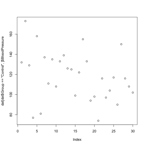
dat[index,]$BloodPressure
 [1] 132 173 129  77 158  81 137 111 135 108 133 139 126 125  99 122 155
[18] 133  94  98  74 116  97 104 117  90 150 116 108 102
Often this operation is written as one line of code:
plot(dat[dat$Group == 'Control',]$BloodPressure)

Challenge - Using logical indexes {.challenge}
- Create a scatterplot showing BloodPressure for subjects not in the control group.
- How many ways are there to index this set of subjects?
Combining Indexing and Assignment
The assignment operator <- can be combined with indexing.
x <- c(1, 2, 3, 11, 12, 13)
x[x < 10] <- 0
x
[1] 0 0 0 11 12 13
Challenge - Updating a subset of values {.challenge}
In this dataset, values for Gender have been recorded as both uppercase
M, Fand lowercasem,f. Combine the indexing and assignment operations to convert all values to lowercase.